Time Series Analysis

4 min readJul 21, 2020

What is Time Series

A time series is a series of data points indexed (or listed or graphed) in time order.

Time Series Data

Time series data is data where one of the columns, usually index, is either days or a particular time stamp for intraday time series. The biggest difference from other data is that we have a specific ordering ie data here is sequential and follows a specific order.

Often, basic regression techniques are not sufficient to grasp the more complex, time-dependent patterns that are common when dealing with time series data. Using time series analysis techniques, the purpose is to get more insight into your data on one hand and to make predictions on the other hand.

Components of Time Series

Seasonality

Seasonality is a characteristic of a time series in which the data experiences regular and predictable changes that recur every calendar year. Any predictable fluctuation or pattern that recurs or repeats over a one-year period is said to be seasonal.

Trend

The trend is the component of a time series that represents variations of low frequency in a time series, the high and medium frequency fluctuations having been filtered out.

Following are the steps to be followed in time series analysis

Step 1: Plot your data, to see if trend and seasonality exists.

Step 2: Check stationary of the data through: “Rolling statistics or Augmented Dickey Fuller Test”.

In Augmented Dickey Fuller Test if p value<0.05 then we can reject the null Hypothesis which says that the time series is not stationary. As we want to make the series stationary we want to get to a point where p<0.05.

Step3: If the data is stationary you can start modeling if not then make it stationary using one of the following ways.

Taking the log transformation
Subtracting the rolling mean
Differencing

Step 4: Plot PACF and ACF Plots and determine the value of p, and q.

Step 5: Use ARIMA Model with these p and q parameters.

Step 6: Forecast.

Here is the code snippet to demonstrate the above mentioned steps.For the airline passengers data.

Read the Data

df=pd.read_csv('airline_passengers.csv')

As you can see there is trend the data is not stationary

Lets use Rolling statistics to check stationarity

#Rolling mean and standard deviation
roll_mean = df.rolling(window=8, center=False).mean()
roll_std = df.rolling(window=8, center=False).std()#plot
plt.figure(figsize=(12,6))
plt.plot(df, color='blue',label='Original')
plt.plot(roll_mean, color='red', label='Rolling Mean')
plt.plot(roll_std, color='black', label = 'Rolling Std')
plt.legend(loc='best')
plt.title('Rolling Mean & Standard Deviation')
plt.show(block=False)

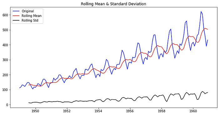
AS you can see the rolling mean is not constant.Hence, data is not stationary

Let's check the stationarity using Dickey-Fuller Test

from statsmodels.tsa.stattools import adfullerdftest = adfuller(df['passengers'])dfoutput = pd.Series(dftest[0:4], index=['Test Statistic', 'p-value', '#Lags Used', 'Number of Observations Used'])for key,value in dftest[4].items():
    dfoutput['Critical Value (%s)'%key] = value
print(dftest)print('Results of Dickey-Fuller Test: \n')
print(dfoutput)

Here are the results for the Dickey fuller test

Results of Dickey-Fuller Test: 

Test Statistic                   0.815369
p-value                          0.991880
#Lags Used                      13.000000
Number of Observations Used    130.000000
Critical Value (1%)             -3.481682
Critical Value (5%)             -2.884042
Critical Value (10%)            -2.578770
dtype: float64

p-value is >0.05 so, the data is not stationary.. Our next step is to make the data stationary.

#Calculating Weighted Moving Average of log transformed data
exp_roll_mean = np.log(df).ewm(halflife=4).mean()#Subtract this exponential weighted rolling mean from the log transformed data
data_minus_exp_roll_mean = np.log(df) - exp_roll_mean#Differencing
data_diff = data_minus_exp_roll_mean.diff(periods=12)

# Drop the missing values
data_diff.dropna(inplace=True)

Here are the results for the stationary check on data_diff

Results of Dickey-Fuller Test: 

Test Statistic                  -3.601666
p-value                          0.005729
#Lags Used                      12.000000
Number of Observations Used    119.000000
Critical Value (1%)             -3.486535
Critical Value (5%)             -2.886151
Critical Value (10%)            -2.579896
dtype: float64

p-value < 0.05 and hence we reject the null hypothesis.The data is stationary.

In my next blog I will talk about time series modeling using ARIMA,SARIMA and FACEBOOK PROPHET.